Half-Step Continuous Block Method for the Solutions of Modeled Problems of Ordinary Differential Equations ()
1. Introduction
We consider the numerical solution of first order initial value problems of the form:
 (1)
(1)
where f is continuous and satisfies Lipchitz’s condition that guarantees the uniqueness and existence of a solution.
Problem in the form (1) has wide application in physical science, engineering, economics, etc. Very often, these problems do not have an analytical solution, and this has necessitated the deviation of numerical schemes to approximate their solutions.
In the past, scholars have developed a continuous linear multistep in solving (1). These authors proposed methods with different basis functions and among them were [1-6] to mention a few.
These authors proposed methods ranging from predictor corrector method to discrete block method.
Scholars later proposed block method. This block method has the properties of Runge-kutta method for being self-starting and does not require development of separate predictors or starting values. Among these authors are [7-12]. Block method was found to be cost effective and gave better approximation.
This paper is divided into sections as follows: Section 1 is the introduction and background of the study; Section 2 contains the discussion about the methodology involved in deriving the continuous multistep method and the continuous block method. Section 3 considers the analysis of the block method in terms of the order, zero stability and the region of absolute stability. Section 4 focuses on the application of the new method on some numeric examples and Section 5 is on the discussion of result. We tested our method on first order ordinary differential equations and compared our result with existing methods.
2. Methodology
Consider power series approximate solution in the form
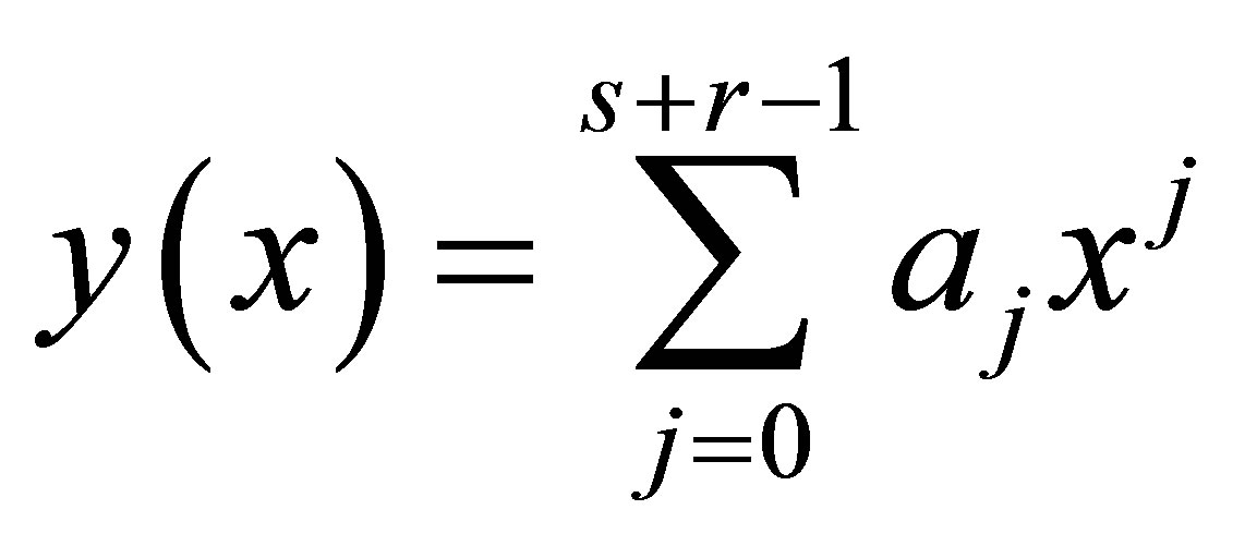 (2)
(2)
where S and r are the number of interpolation and collocation points respectively.
The first derivative of (2) gives
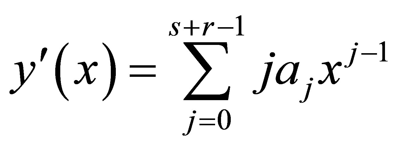 (3)
(3)
Substituting (3) into (2) gives
 (4)
(4)
Collocating (3) at  and interpolating
(2) at  gives a system of non-linear equation in the form
 (5)
(5)
where
 ,
, 
Solving (5) for the ajs and substituting back into (4) gives a continuous multistep method in the form
 (6)
(6)
where a0 = 1 and the coefficients of  gives
gives


where  Solving (6) for the independent solution gives a continuous block method in the form
 (7)
(7)
where  is the order of the differential equation s is the collocation points. Hence the coefficient of
  in (7)


where 
Evaluating (2.5) at  gives a discrete block formula of the form
 (8)
(8)
where  matrix where


3. Analysis of the Basic Properties of Our New Method
3.1. Order of the Method
Let the linear operator  associated with the block formular be defined as
 (9)
(9)
expanding in Taylor series and comparing the coefficient of h gives
 (10)
(10)
Definition:-The linear operator L and the associated continuous linear multistep method (3.1) are said to be of order p if  is called the error constant and implies that the local truncation error is given by
For our method;

Expanding in Taylor series expansion gives


Equating coefficients of the Taylor series expansion to zero yield

Hence we arrived at a uniform order 6 for our method with error constants

3.2. Zero Stability
Definition: The block (8) is said to be zero stable, if the roots Zs,  of the characteristic polynomial
  defined by
  satisfies
  and every root satisfying
  have multiplicity not exceeding the order of the differential equation. Moreover as
  where
where  is the order of the differential equation, r is the order of the matrix
  and E.
For our method

 Hence our method is zero stable.
3.3 Region of Absolute Stability
The block formulated as a general linear method where it is partition in the form

The elements of  and
and  are obtained from the coefficients of the collocation points,
  and
and  are obtained from the interpolation points.
Applying the test equation  leads to the recurrence equation

The stability function is given by

and the stability polynomial of the method is given as
The region of absolute stability of the method is defined as 
For our method, writing the block in partition form gives

4. Real Life Problems
4.1. Problem 1: (SIR MODEL)
The SIR model is an epidemiological model that computes the theoretical numbers of people infected with a contagious illness in a closed population over time. The name of this class of models derives from the fact that they involves coupled equations relating the number of susceptible people S(t), number of people infected I(t) and the number of people who have recovered R(t). This is a good and simple model for many infectious diseases including measles, mumps and rubella [13-15]. The SIR model is described by the three coupled equations.
 (11)
(11)
 (12)
(12)
 (13)
(13)
where  are positive parameters. Define
  to be
to be
 (14)
(14)
Adding Equations (11)-(13), we obtain the following evolution equations for 
 (15)
(15)
Taking  and attaching an initial condition
  (for a particular closed population), we obtain,
 (16)
(16)
whose exact solution is,
 (17)
(17)
Applying our new half step numerical scheme (8) to solve SIR model simplified as (17) gives results as shown in Table 1.
4.2. Problem 2 (Growth Model)
Let us consider the differential equation of the form;
 (18)
(18)
Equation (18) represents the rate of growth of bacteria in a colony. We shall assume that the model grows continuously without restriction. One may ask; how many bacteria are in the colony after some minutes if an individual produces an offspring at an average growth rate of 0.2? We also assume that  is the population size at time
  (Table 2).
The theoretical solution of (18) is given by;
s (19)
Note that, growth rate  in (18).

Table 1. Showing results for SIR model problem.

Table 2. Showing results for growth model problem.
Applying our new half step numerical scheme (8) to solve the Growth model (17) gives results as shown in Table 2 [16].
4.3. Problem 3 (Decay Model)
A certain radioactive substance is known to decay at the rate proportional to the amount present. A block of this substance having a mass of 100 g originally is observed. After 40 mins, its mass reduced to 90 g. Find an expression for the mass of the substance at any time and test for the consistency of the block integrator on this problem for .
.
The problem has a differential equation of the form;
 (21)
(21)
where N represents the mass of the substance at any time  is a constant which specifies the rate at which this particular substance decays. Note that,

Since for any growth/decay problem,


Thus, the theoretical solution to (20) is given by,
 (22)
(22)
which is also the expression for the mass of the substance at any time t.
Applying our new half step numerical scheme (8) to solve the Growth model (22) gives results as shown in Table 3 [16,17] (Table 3).
5. Discussion of the Result
We have considered three real-life model problems to test the efficiency of our method. Problems 1 and 2 and 3 were solved by Sunday et al. [17]. They proposed an order six block integrator for the solution of first-order ordinary differential equations. Our half-step block method gave better approximation as shown in Tables

Table 3. Showing results for decay model problem.

Figure 1. Showing region of absolute stability of our method.
1-3 because the iteration per step in the new method was lower than the method proposed by [17]. Our method was found to be zero stable, consistent and converges. Figure 1 shows the region of absolute stability. From the numerical examples, we could safely conclude that our method gave better accuracy than the existing methods.