Exponential Attractors of the Nonclassical Diffusion Equations with Lower Regular Forcing Term ()

1. Introduction
We consider the asymptotic behavior of solutions to be the following nonclassical diffusion equation:
 (1.1)
(1.1)
where  is a bounded domain with smooth boundary
 , and the external forcing term
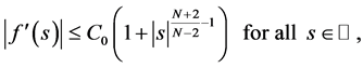
 , non-linear function
  with
with  and satisfies the following conditions:
 (1.2)
(1.2)
and
 (1.3)
(1.3)
where  is a positive constant and
  is the first eigenvalue of
  on
on . The number
  is called the critical exponent; since the nonlinearity
  is not compact in this case, this is one of the essential difficulties in studying the asymptotic behavior.
This equation appears as a nonclassical diffusion equation in fluid mechanics, solid mechanics and heat conduction theory, see for instance [1] -[3] and the references therein.
Since Equation (1.1) contains the term , it is different from the usual reaction diffusion equation essentially. For example, the reaction diffusion equations has some smoothing effect, that is, although the initial data only belongs to a weaker topology space, the solution will belong to a stronger topology space with higher regularity. However, for Equation (1.1), if the initial data
  belongs to
 , the solution
  with
with  is always in
  and has no higher regularity because of
 , which is similar to the hyperbolic equation. Consequently, its dynamics would be more complex and interesting.
The long-time behavior of the solutions of (1.1) has been considered by many researchers; see, e.g. [4] -[9] , and the references therein. For instance, for the case , the existence of a global attractor of (1.1) in
  was obtained in [4] under the assumptions that
  satisfies (1.2) and (1.3) corresponding to
and the additional condition  with
with , which essentially requires that the nonlinearity is subcritical. In [7] the authors investigated the existence of the global attractors for
 , and proved the asymptotic regularity and existence of exponential attractors for
  only under the conditions (1.2)-(1.3). Recently, the authors in [9] showed the asymptotic regularity of solutions of Equation (1.1) in
  for any
  and for
 ,
,  only under the assumptions (1.2)-(1.3).
For the limit of our knowledge, the existence of exponential attractors of Equation (1.1) has not been achieved by predecessors for . On the other hand, we note that in [10] the authors scrutinized the asymptotic regularity of the solutions for a semilinear second order evolution equation when
 , and based on this regularity, they constructed a family of finite dimensional exponential attractors. However, they require the following additional technical assumptions besides (1.2) and (1.3):

and

In this article, motivated by the work in [10] -[12] , based on the asymptotic regularity in [9] , we construct a finite dimensional exponential attractor of (1.1) only under the conditions (1.2) and (1.3).
Our main result is Theorem 1.1 Assume  and satisfies (1.2)-(1.3),
 . Then the semigroup
  associated with problem (1.1) has an exponential attractor
  in
in .
.
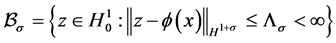
Remark 1.1 If  is a global attractor of (1.1) in
 , we know that
 , then Theorem 1.1 implies that fractal dimension of the global attractor
  is finite.
2. Notations and Preliminaries
In this section, for convenience, we introduce some notations about the functions space which will be used later throughout this article.
•  with domain
 , and consider the family of Hilbert space
  with the standard inner products and norms, respectively,
Especially,  means the
  inner product and norm, respectively.
•  with the usual norm
 . Especially, we denote
  and
and .
.
•  are continuous increasing functions.
•  denote the general positive constants,
  , which will be different from line to line.
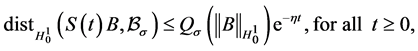
We also need the following the transitivity property of exponential attraction, e.g., see [[12] , Theorem 5.1]:
Lemma 2.1 ([13] ) Let  be subsets of
  such that

for some  and
and . Assume also that for all
  there holds

for some  and
and . Then it follows that

where  and
and .
.
3. Exponential Attractor
In this subsection, based on the asymptotic regularity obtained in [9] , we will construct an exponential attractor by the methods and techniques devised in [10] -[12] . We first need the following Lemmas:
Lemma 3.1 ([7] ) Let  satisfies (1.2)-(1.3) and
 . Then for any
  and any
 , there is a unique solution
  of (1.1) such that

Moreover,the solution continuously depends on the initial data in .
.
In the remainder of this section, we denote by  the semigroup associated with the solutions of (1.1)-(1.3).
Lemma 3.2 ([7] ) Under conditions of above Lemma, There is a positive constant  such that for any bounded subset
 , there exists
  such that
 (3.1)
(3.1)
From this Lemma, we know that the semigroup of operators  generalized by (1.1) possesses a bounded absorbing set
  in
in .
.
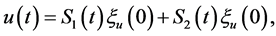
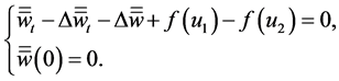
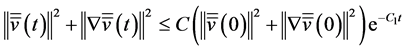
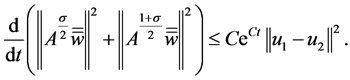
Lemma 3.3 Under conditions of , and
, and  be two solutions of (1.1) with
 , respectively, it follows that
 (3.2)
(3.2)
Proof Let  satisfies the following equation
 (3.3)
(3.3)
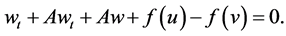
Taking the scalar product of (3.3) with , we find,
 (3.4)
(3.4)
From the condition (1.2), by using the Hölder inequality, and noting the embedding , we have
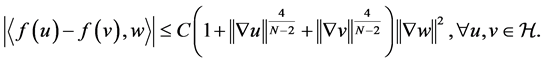
And then, by means of (3.1), we obtain
 (3.5)
(3.5)
So, combining with Equation (3.4), (3.5), we get
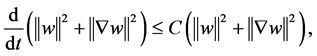
then using the Gronwall lemma to above inequality, we can conclude our lemma immediately.
Lemma 3.4 ([9] ) Let  and satisfies (1.2), (1.3),
 . Then, for any
 , there exists a subset
 , a positive constant
  and a monotone increasing function
 such that for any bounded set
 ,
,
 (3.6)
(3.6)
where  and
and  depend on
  but
but  is independent of
 ;
;  satisfying
 (3.7)
(3.7)
for some positive constant ; And
; And  is the unique solution of the following elliptic equation
 (3.8)
(3.8)
where the constant  such that
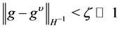 . Furthermore, we know that the solution
  only belongs to
  when
when  satisfies (1.2)-(1.3).
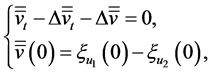
Lemma 3.5 ([9] ) Under the assumption of Lemma 3.4, for any bounded subset , if the initial data
 , then the solution
  of (1.1) has the following estimates similar to (3.7) in Lemma 3.4, more precisely, we have
 (3.9)
(3.9)
where the constant  depends only on
  and the
  -bound of
 .
.
Lemma 3.6 There exists  such that
 (3.10)
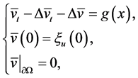
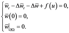
Proof For the solution  of (1.1), we now decompose
  as follows
 (3.11)
where  is a fixed solution of (3.8), and
  satisfies the following equation :
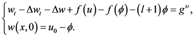 (3.12)
At the same time, noticing the embedding , and from Lemma 3.5 we yield
 (3.13)
Taking the inner product of (3.12) with , we get
 (3.14)
By means of (3.1) and (3.13) and together with H lder, Young inequalities, it follows that
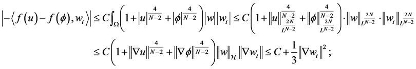 (3.15)

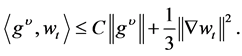
Thus, combining with (3.14), there holds

Integrating the above inequality on  and noting
 , the proof completes.
Next, we will prepared for constructing an exponential attractor of  in
in  by applying the abstract results devised in [10] -[12] [14] .
Firstly, for each fixed , we define
 (3.16)
where  is the set obtained in Lemma 3.4. Then, from Lemma 3.5 we know that
 (3.17)
Secondly, let us establish some properties of this set.
•  is a compact set in
 , due to Lemma 3.4.
•  is positive invariant. In fact, from the continuity of
 , we have
 (3.18)
• There holds
 (3.19)
Indeed, it is apparent that
 (3.20)
Hence, (3.19) follows from Lemma 2.1.
• There is  such that
 (3.21)
This is a direct consequence of Lemma 3.6.
Therefore such a set  is a promising candidate for our purpose.
Finally, we need the following two lemmas.
Lemma 3.7 For every , the mapping
  is Lipschitz continuous on
 .
.
Proof For  and
and  we have
 (3.22)
The first term of the above inequality is handled by estimate (3.2). Concerning the second one,
 (3.23)
Hence, there exists a constant , such that
 (3.24)
On the other hands, for each initial data , we can decompose the solution
  of (1.1) as
 (3.25)
where 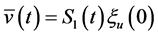 and
and  solve the following equations respectively:
 (3.26)
and
 (3.27)
Therefore, we will have the following lemma:
Lemma 3.8 The following two estimates hold:
 (3.28)
and
 (3.29)
where the constant  depends only on
  and
and .
.
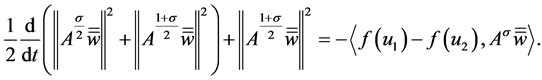
Proof Given two solutions  of Equation (1.1) origination from
 , respectively.
Set

where  and
and  solve the following equations respectively:
 (3.30)
and
 (3.31)
It is apparent that  and
and 
Taking the product of (3.30) with  in
in , we get
 (3.32)
So
 (3.33)
Hence, setting
 (3.34)
we have

So, we obtain the result (3.28).
On the other hands, taking the product of (3.31) with  in
in , we ge
 (3.35)
Since , we have
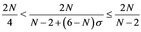 .
.
So, from (1.2) and using H lder inequality, we have
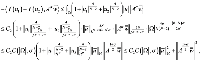 (3.36)
where the constant  comes from the embedding
 ,
, .
.
From Lemma 3.3, we obtain the inequality
and an integration on , we can get the estimate (3.29).
Proof of Theorem 1.1 Applying the abstract results devised in [10] -[12] , from Lemma 3.7 and Lemma 3.8, we can prove the existence of an exponential attractor  for
for  in
in  immediately.
Remark 3.9 As a direct consequence of Theorem 1.1 and the a priori estimates given in [[9] , Lemma 3.5] and Lemma 3.8, we decompose  as
as , where
  is bounded in
  for any
 and
and  is the unique solution of (3.8).
Acknowledgements
The authors thank the referee for his/her comments and suggestions, which have improved the original version of this article essentially. This work was partly supported by the NSFC (11061030,11101334) and the NSF of Gansu Province(1107RJZA223), in part by the Fundamental Research Funds for the Gansu Universities.
NOTES
*Corresponding author.