Limit Cycle Bifurcations in a Class of Cubic System near a Nilpotent Center ()
1. Introduction
In the International Congress of Mathematics held in Paris in 1900, Hilbert made a list of 23 problems. The second part of Hilbert’s 16th problem is still an open and difficult question: to find a upper bound of the number of limit cycles and their relative locations in polynomial vector fields of order n.
If the singular point of the system is a non-saddle, nor nilpotent, the related Hopf bifurcations are elementary, see [1-3] and their references. Hopf bifurcations from the elementary focus type of singularities have found broad and important applications in biology, chemistry and physics and engineering, see [4-7] for examples. Yet for the bifurcation of limit cycles from a non-elementary center in a more general planar vector field, its intrinsic dynamics is still far away from understanding due to the complexity and technical difficulties in dealing with such bifurcations.
Then it was natural to restrict the study of the nilpotent center by assuming the system is a perturbation of a Hamiltonian system. Consider the following system
 (1.1)
(1.1)
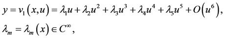
where ,
,  and
and  are
are  functions,
  is small and
  with D a compact set.
When , system (1.1) becomes
 (1.2)
(1.2)
which is Hamiltonian system. Now suppose that the Hamiltonian system (1.2) has a nilpotent center at the origin, namely the function H satisfies the following conditions:
(H1)  is a
is a  function, satisfying
 ;
;
(H2) , the equation
  defines a closed curve Lh surrounding the origin and Lh approaches the origin as h goes to zero;
(H3)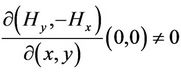 ,
, .
.
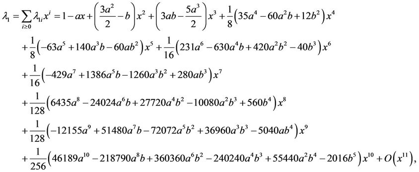
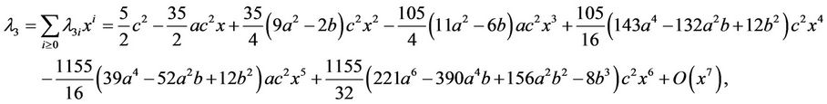
It follows that the expansion of H at the origin has the form

Assume that the equation  intersects the positive x-axis at
 . Let
. Let  denote the first intersection point of the positive orbit of (1.1) starting at
  with the positive x-axis. Then, we have
 (1.3)
(1.3)
where
 (1.4)
(1.4)
The Abelian integral M above is called the first order Melnikov function of system (1.1). From Han [8], we have a general theorem as follows.
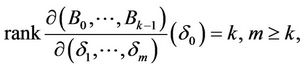
Theorem 1.1. Suppose that the origin is nilpotent singular point  and that
  approaches the origin as h goes to zero. If there exist an integer
  and
and  such that

and
then we have 1)  has at most k zeros near
  for
for  and all
  near
near , and k zeros can appear for some
  near
near .
.
2) System (1.1) has at least k limit cycles near the origin for some  near
near .
.
2. Main Results and Proof
Consider the following near-Hamiltonian system:
 (2.1)
(2.1)
where  and p and q are cubic polynomials. We can write
 (2.2)
(2.2)
Then unperturbed system  is a Hamiltonian system with Hamiltonian
 (2.3)
(2.3)
system  has a nilpotent center at the origin. Let
  be the closed curve defined by
 . Then it can be presented as
 (2.4)
(2.4)
Assume that the positive solution of the above equation in y is
 (2.5)
(2.5)
where 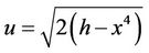 and
and . Then by (2.4) and (2.5) we obtain


By [8] the negative solution of (2.4) in y satisfies . Thus, two solutions of (2.4) are
 (2.6)
(2.6)
On the other hand, the intersection points of Lh and xaxis have the x-coordinates  and
and . Then by (2.2) we can write
 (2.7)
(2.7)
where
 (2.8)
(2.8)
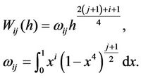
Here,

Introduce
 (2.9)
(2.9)
Then, similar to the method of Han [8] we have
 (2.10)
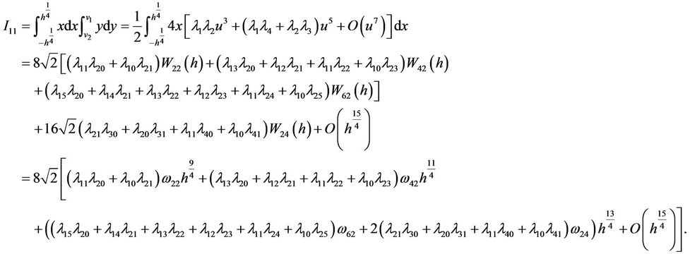
Therefore, in turn by (2.6)-(2.10) we have


Noting that , then similarly we have

In the same way, using , we have

Hence, we have

where 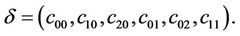 And
And


Now it is direct that

Here, if let ,
,  ,
,  , then for some cubic system (2.1) we can obtain the above determinant is not zero, then the function M can have 5 simple zeros in h > 0 near h = 0 for some
  near
near . For example, let
 ,
,  ,
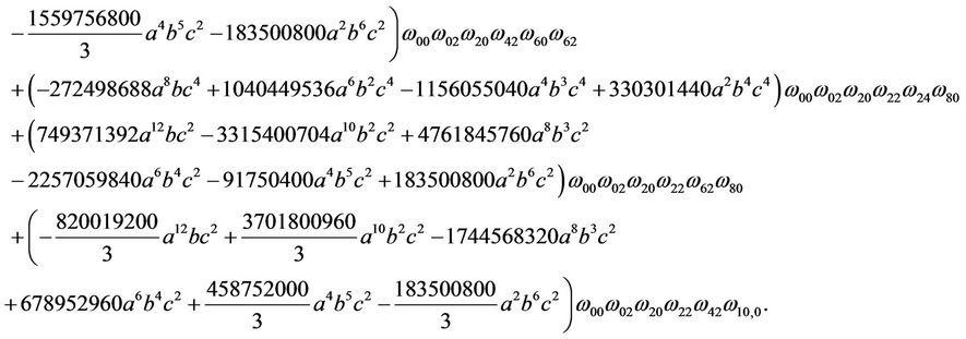
,  , we obtain from the above formula

Here,


then we can obtain
 (2.11)
By Theorem 1.1 we have:
Theorem 2.1. The function  has at most 5 zeros in
  near
near , and for
  small the cubic system (2.1) can have 5 limit cycles near the origin.
NOTES