Reliability Modelling and Analysis of Redundant Systems Connected to Supporting External Device for Operation Attended by a Repairman and Repairable Service Station ()
1. Introduction
High system reliability and availability play a vital role towards industrial growth as the profit is directly dependent on production volume which depends upon system performance. Thus the reliability and availability of a system may be enhanced by proper design, optimization at the design stage and by maintaining the same during its service life. Because of their prevalence in power plants, manufacturing systems, and industrial systems, many researchers have studied reliability and availability problem of different systems (see, for instance, Ref [1] -[8] and the references therein). In real-life situations we often encounter cases where the systems that cannot work without the help of external supporting devices connect to such systems. These external supporting devices are systems themselves that are bound to fail. Where such systems exist, a repairable service station is provided for the immediate repair of failed unit. Such systems are found in power plants, manufacturing systems, and industrial systems. Ref [9] [10] performed comparative analysis of some reliability characteristics between redundant systems requiring supporting units for their operation.
The problem considered in this paper is different from the work of Ref [9] [10] . The objectives of the present paper are three. The first is to develop the explicit expressions for the mean time to system failure (MTSF) and steady- state availability. The second objective is to perform a parametric investigation of various system parameters on mean time to system failure (MTSF) and steady-state availability and capture their impact on the mean time to sys- tem failure (MTSF) and steady-state availability. The third objective is to perform comparative analysis between the three configurations based on assumed numerical values in order to determine the optimal configuration.
2. Description of the Systems
We consider three redundant systems connected to an external supporting device for their operation as follows. The first system is a 2-out-of-3 system connected to a supporting device and has a repairable service station. The second is also a 2-out-of-3 system connected to supporting device and has two standby repairable service stations. The third system is a 3-out-of-4 system connected to a supporting device and has a repairable service station. We assume that switching is perfect and instantaneous. We also assume that two units cannot fail simultaneously. Whenever a unit fails with failure rate , it is immediately sent to a service station for repair with service rate
 . However, on the course of repairing failed unit, the service is bound to fail with failure rate of
  and service rate of
  and failed unit must wait whenever the service station is under repair for first and third system, while the standby service will continue repairing failed unit for the second system. The supporting device is a system that is prone to failure. Whenever the supporting device failed with rate
  it is attended by a repairman, the system stop working and must wait until the supporting device is repaired with rate
 .
.
3. Mean Time to System Failure Models Formulation
3.1. MTSF Formulation for Configuration I
For configuration I, we define  to be the probability that the system at time
  is in state
 . Also let
  be the probability row vector at time
 , we have the following initial condition:

We obtain the following differential equations:
 (1)
(1)
This can be written in the matrix form as
 (2)
(2)
where
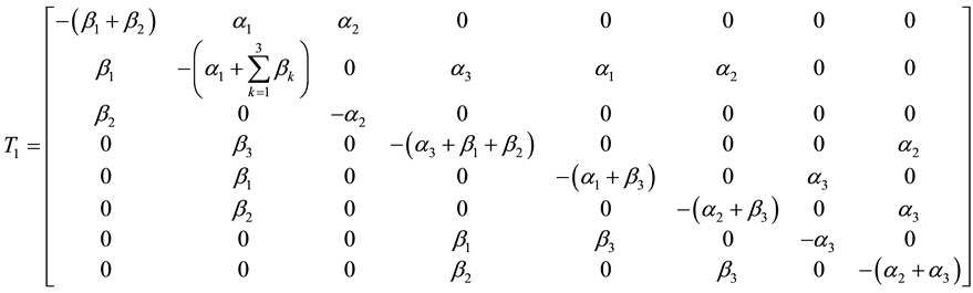
It is difficult to evaluate the transient solutions, the procedure to develop the explicit expression for  is to delete the rows and column of absorbing states of matrix
 ![]() and take the transpose to produce a new matrix, say
and take the transpose to produce a new matrix, say![]() . Following Ref [11] [12] , the expected time to reach an absorbing state is obtained from
. Following Ref [11] [12] , the expected time to reach an absorbing state is obtained from
![]() (3)
(3)
where
![]()
![]()
![]()
3.2. MTSF Formulation for Configuration II
For configuration II, we define ![]() to be the probability that the system at time
to be the probability that the system at time ![]() is in state
is in state![]() . Also let
. Also let ![]() be the probability row vector at time
be the probability row vector at time![]() , we have the following initial condition:
, we have the following initial condition:
![]()
The differential equations are expressed in the form
![]() (4)
(4)
where
![]()
and
![]()
Using the procedure described in Subsection 3.1, the expected time to reach an absorbing state is
![]() (5)
(5)
where
![]()
![]()
![]()
3.3. MTSF Formulation for Configuration III
For configuration II, we define ![]() to be the probability that the system at time
to be the probability that the system at time ![]() is in state
is in state![]() . Also let
. Also let ![]() be the probability row vector at time
be the probability row vector at time![]() , we have the following initial condition:
, we have the following initial condition:
![]()
The differential equations are expressed in the form
![]() (6)
(6)
where
![]()
Using the procedure described in Subsection 3.1, the expected time to reach an absorbing state is
![]() (7)
(7)
where
![]()
![]()
![]()
4. Availability Models Formulation
4.1. Availability Model Formulation for Configuration I
For the analysis of availability case of configuration I we use the same initial condition as in Subsection 3.1
![]()
The differential equations above are expressed in the form
![]()
The steady-state availability is given by
![]() (8)
(8)
In the steady-state, the derivatives of the state probabilities become zero and therefore Equation (2) become
![]() (9)
(9)
which is in matrix form
![]()
Using the following normalizing condition
![]() (10)
(10)
Substituting (10) in the last row of (9) to compute the steady-state probabilities, the expression for steady- state availability is given by
![]() (11)
(11)
![]()
![]()
4.2. Availability Model Formulation for Configuration II
For the analysis of availability case of configuration II we use the same initial condition as in Subsection 3.2
![]()
The differential equations are expressed in the form
![]()
The steady-state availability is given by
![]() (12)
(12)
In the steady-state, the derivatives of the state probabilities become zero and therefore Equation (4) become
![]() (13)
(13)
which is in matrix form
![]()
Using the following normalizing condition
![]() (14)
(14)
Substituting (14) in the last row of (13) to compute the steady-state probabilities, the expression for steady- state availability is given by
![]() (15)
(15)
![]()
![]()
4.3. Availability Model Formulation for Configuration III
For the analysis of availability case of configuration III we use the same initial condition as in Subsection 3.3
![]()
The differential equations are expressed in the form
![]()
The steady-state availability is given by
![]() (16)
(16)
In the steady-state, the derivatives of the state probabilities become zero and therefore Equation (6) become
![]() (17)
(17)
which is in matrix form
![]()
Using the following normalizing condition
![]() (18)
(18)
Substituting (18) in the last row of (17) to compute the steady-state probabilities, the expression for steady- state availability is given by
![]() (19)
(19)
![]()
![]()
5. Comparison of the Three Configurations
In this section, we numerically compare the results for availability and MTSF for the developed models for the three configurations.
Case I:
We fix![]() ,
, ![]() ,
, ![]() ,
, ![]() ,
, ![]() and vary
and vary ![]() between 0 to 1 for Figure 1,
between 0 to 1 for Figure 1, ![]() ,
, ![]() ,
, ![]() ,
, ![]() ,
, ![]() and vary
and vary ![]() between 0 to 1 for Figure 2.
between 0 to 1 for Figure 2.
Case II:
We fix![]() ,
, ![]() ,
, ![]() ,
, ![]() ,
, ![]() and vary
and vary ![]() between 0 to 1 for Figure 3 and
between 0 to 1 for Figure 3 and![]() ,
, ![]() ,
, ![]() ,
, ![]() ,
, ![]() and vary
and vary ![]() between 0 to 1 for Figure 4.
between 0 to 1 for Figure 4.
Case III:
We fix![]() ,
, ![]() ,
, ![]() ,
, ![]() ,
, ![]() and vary
and vary ![]() between 0 to 1 for Figure 5 and
between 0 to 1 for Figure 5 and![]() ,
, ![]() ,
, ![]() ,
, ![]() ,
, ![]() and vary
and vary ![]() between 0 to 1 for Figure 6.
between 0 to 1 for Figure 6.
Case IV:
We fix![]() ,
, ![]() ,
, ![]() ,
, ![]() and vary
and vary ![]() between 0 to 1 for Figure 7,
between 0 to 1 for Figure 7, ![]() ,
, ![]() ,
, ![]() ,
, ![]() and vary
and vary ![]() between 0 to 1 for Figure 8 and
between 0 to 1 for Figure 8 and![]() ,
, ![]() ,
, ![]() ,
, ![]() and vary
and vary ![]() between 0 to 1 for Figure 9, and vary
between 0 to 1 for Figure 9, and vary ![]() and
and ![]() for Figures 9-11.
for Figures 9-11.
From Figure 1, the availability results for the three systems being studied against the repair rate![]() . It is
. It is
clear from the Figure that configuration II has higher availability with respect to ![]() as compared with the other two configurations. There is slight difference between the availability of configuration II and that of configuration III with respect to
as compared with the other two configurations. There is slight difference between the availability of configuration II and that of configuration III with respect to![]() . These tend to suggest that configuration II is better than the other configurations. Figure 2 depicts the availability calculations for the three configurations against
. These tend to suggest that configuration II is better than the other configurations. Figure 2 depicts the availability calculations for the three configurations against![]() . The observations that can be made here are much similar to those made on Figure 1. From Figure 1 and Figure 2, it is clear that
. The observations that can be made here are much similar to those made on Figure 1. From Figure 1 and Figure 2, it is clear that![]() .
.
However, one can say that the results from Figure 3 show slight distinction between availability of three configurations with respect to![]() . The differences between availability of configuration II and the other two configurations slightly increase as
. The differences between availability of configuration II and the other two configurations slightly increase as ![]() increases. There is significant difference between the three configurations with respect to
increases. There is significant difference between the three configurations with respect to ![]() in Figure 4. It is evident from Figure 4 that configurations II and III have higher availabili-
in Figure 4. It is evident from Figure 4 that configurations II and III have higher availabili-
ty than configuration I as ![]() increases. Thus,
increases. Thus, ![]() for Figure 3 and
for Figure 3 and ![]() for Figure 4.
for Figure 4.
Results from Figure 5 and Figure 6 show slight distinction between availability of three configurations with respect to ![]() and
and![]() . The differences between availability of configuration II and the other two configurations widen as
. The differences between availability of configuration II and the other two configurations widen as ![]() and
and ![]() increases respectively. It is evident from Figure 5 and Figure 6 that configurations
increases respectively. It is evident from Figure 5 and Figure 6 that configurations
II has higher availability than configuration I and III as ![]() and
and ![]() increases. Thus,
increases. Thus,![]() .
.
Simulations of MTSF for the three configurations depicted in Figures 7-9 show that MTSF increases as ![]() and
and![]() , and decreases as
, and decreases as ![]() increases for any configuration. It is clear from these Figures that differences between MTSF of configuration I and III and configuration II widen as
increases for any configuration. It is clear from these Figures that differences between MTSF of configuration I and III and configuration II widen as![]() ,
, ![]() and
and ![]() increases respectively. It is evident from these Figures that configuration I and III have equal MTSF higher than configuration II as
increases respectively. It is evident from these Figures that configuration I and III have equal MTSF higher than configuration II as![]() ,
, ![]() and
and ![]() increases. Figure 10 and Figure 11 show that the MTSF decreases as
increases. Figure 10 and Figure 11 show that the MTSF decreases as ![]() and
and ![]() for any configuration. It is evident from Figure 10 and Figure 11 that configurations I has higher MTSF than configuration II and III as
for any configuration. It is evident from Figure 10 and Figure 11 that configurations I has higher MTSF than configuration II and III as ![]() and
and ![]() increases. Thus, from Figures 7-9, configuration I and II have equal MTSF. From Figure 10 the optimal configuration is configuration I while in Figure 11, configuration I and II have equal MTSF.
increases. Thus, from Figures 7-9, configuration I and II have equal MTSF. From Figure 10 the optimal configuration is configuration I while in Figure 11, configuration I and II have equal MTSF.
6. Conclusion
In this paper, we studied the reliability characteristics of three dissimilar systems connected supporting device. We developed the explicit expressions for steady-state availability and mean time to system failure (MTSF) for each configuration and performed comparative analysis numerically to determine the optimal configuration. It is evident from Figures 1-6 that configuration II is optimal configuration using steady-state availability while using MTSF, the optimal configuration depends on the values of![]() ,
, ![]() ,
, ![]() ,
, ![]() and
and![]() . The present study will help the engineers and designers to develop sophisticated models and to design more critical system in interest of human kind.
. The present study will help the engineers and designers to develop sophisticated models and to design more critical system in interest of human kind.